I – Short answer: use powerlog in Stata
II – Long answer:
powerlog, p1(.25) p2(.35) rsq(.4)
In order to understand that, you should think of a ‘dependent variable’, ‘key predictor’, and all other predictors which are of less interest, or confounders.
p1 and p2 concern the key predictor and the dependent variable (Y) only:
rsq concerns only the key predictors and all other predictors. Ideally there should be no endogenous variable in the set of predictors – or rsq should be 0. If you expect some level of correlation between the key predictor and other predictors, note that:
In the case above p1 is set at 0.25 and p2 at 0.35. That means when the key predictor takes its mean value, the possibility that Y=1 (eg. getting promoted, getting cancer, being an alcohol abuser) is 0.25. Note that when p2 is set at 0.35, the expected association between Y and key predictor is a positive one – when key predictor increase, the change of getting Y=1 increases.
In Stata we get 290 for power=.80
powerlog, p1(.25) p2(.35) rsq(.4)
Logistic regression power analysis
One-tailed test: alpha=.05 p1=.25 p2=.35 rsq=.4 odds ratio=1.615384615384615
power n
0.60 173
0.65 196
0.70 223
0.75 253
0.80 290
0.85 335
0.90 397
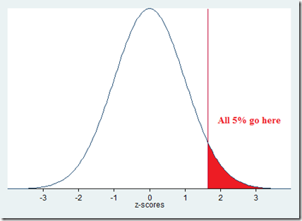
Note that this is a power analysis for one-tailed test, which mean 5% chance of ‘wrong guess’ goes all on one tail of the curve:

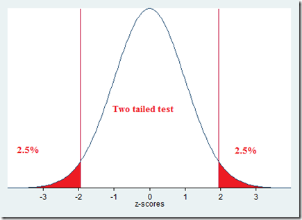
For a two-tailed test, each tail would have a 2.5% chance that the guess would go wrong

In stata, we can do as below. This time we get 369 for power=.8, two tailed.
. powerlog, p1(.25) p2(.35) rsq(.4) alpha(0.025)
Logistic regression power analysis
One-tailed test: alpha=.025 p1=.25 p2=.35 rsq=.4 odds ratio=1.615384615384615
power n
0.60 235
0.65 263
0.70 293
0.75 328
0.80 369
0.85 420
0.90 489
II – Long answer:
powerlog, p1(.25) p2(.35) rsq(.4)
In order to understand that, you should think of a ‘dependent variable’, ‘key predictor’, and all other predictors which are of less interest, or confounders.
p1 and p2 concern the key predictor and the dependent variable (Y) only:
- at p1, you guess the possibility of Y=1 if p1 is at its mean
- at p2, you guess the possibility of Y=1 if p1 is at its mean plus one standard deviation (or p1=mean+1 SD)
rsq concerns only the key predictors and all other predictors. Ideally there should be no endogenous variable in the set of predictors – or rsq should be 0. If you expect some level of correlation between the key predictor and other predictors, note that:
- strong correlation: 0.5 to 1
- moderate correlation 0.3 to 0.49
- weak correlation 0.1 to 0.29
In the case above p1 is set at 0.25 and p2 at 0.35. That means when the key predictor takes its mean value, the possibility that Y=1 (eg. getting promoted, getting cancer, being an alcohol abuser) is 0.25. Note that when p2 is set at 0.35, the expected association between Y and key predictor is a positive one – when key predictor increase, the change of getting Y=1 increases.
In Stata we get 290 for power=.80
powerlog, p1(.25) p2(.35) rsq(.4)
Logistic regression power analysis
One-tailed test: alpha=.05 p1=.25 p2=.35 rsq=.4 odds ratio=1.615384615384615
power n
0.60 173
0.65 196
0.70 223
0.75 253
0.80 290
0.85 335
0.90 397
Note that this is a power analysis for one-tailed test, which mean 5% chance of ‘wrong guess’ goes all on one tail of the curve:

For a two-tailed test, each tail would have a 2.5% chance that the guess would go wrong

In stata, we can do as below. This time we get 369 for power=.8, two tailed.
. powerlog, p1(.25) p2(.35) rsq(.4) alpha(0.025)
Logistic regression power analysis
One-tailed test: alpha=.025 p1=.25 p2=.35 rsq=.4 odds ratio=1.615384615384615
power n
0.60 235
0.65 263
0.70 293
0.75 328
0.80 369
0.85 420
0.90 489