Indochina films

Films on Indochina,

http://www.britishpathe.com/search/query/IndoChina

Marginal effect

How to choose a statistical test in a software?

What statistical analysis should I use?

The following table shows general guidelines for choosing a statistical analysis. We emphasize that these are general guidelines and should not be construed as hard and fast rules. Usually your data could be analyzed in multiple ways, each of which could yield legitimate answers. The table below covers a number of common analyses and helps you choose among them based on the number of dependent variables (sometimes referred to as outcome variables), the nature of your independent variables (sometimes referred to as predictors). You also want to consider the nature of your dependent variable, namely whether it is an interval variable, ordinal or categorical variable, and whether it is normally distributed (see What is the difference between categorical, ordinal and interval variables? for more information on this). The table then shows one or more statistical tests commonly used given these types of variables (but not necessarily the only type of test that could be used) and links showing how to do such tests using SAS, Stata and SPSS.

Number of Dependent Variables	Nature of Independent Variables	Nature of Dependent Variable(s)	Test(s)	How to SAS	How to Stata	How to SPSS
1	0 IVs (1 population)	interval & normal	one-sample t-test	SAS	Stata	SPSS
		ordinal or interval	one-sample median	SAS	Stata	SPSS
		categorical (2 categories)	binomial test	SAS	Stata	SPSS
		categorical	Chi-square goodness-of-fit	SAS	Stata	SPSS
	1 IV with 2 levels (independent groups)	interval & normal	2 independent sample t-test	SAS	Stata	SPSS
		ordinal or interval	Wilcoxon-Mann Whitney test	SAS	Stata	SPSS
		categorical	Chi-square test	SAS	Stata	SPSS
			Fisher's exact test	SAS	Stata	SPSS
	1 IV with 2 or more levels (independent groups)	interval & normal	one-way ANOVA	SAS	Stata	SPSS
		ordinal or interval	Kruskal Wallis	SAS	Stata	SPSS
		categorical	Chi-square test	SAS	Stata	SPSS
	1 IV with 2 levels (dependent/matched groups)	interval & normal	paired t-test	SAS	Stata	SPSS
		ordinal or interval	Wilcoxon signed ranks test	SAS	Stata	SPSS
		categorical	McNemar	SAS	Stata	SPSS
	1 IV with 2 or more levels (dependent/matched groups)	interval & normal	one-way repeated measures ANOVA	SAS	Stata	SPSS
		ordinal or interval	Friedman test	SAS	Stata	SPSS
		categorical	repeated measures logistic regression	SAS	Stata	SPSS
	2 or more IVs (independent groups)	interval & normal	factorial ANOVA	SAS	Stata	SPSS
		ordinal or interval	ordered logistic regression	SAS	Stata	SPSS
		categorical	factorial logistic regression	SAS	Stata	SPSS
	1 interval IV	interval & normal	correlation	SAS	Stata	SPSS
		interval & normal	simple linear regression	SAS	Stata	SPSS
		ordinal or interval	non-parametric correlation	SAS	Stata	SPSS
		categorical	simple logistic regression	SAS	Stata	SPSS
	1 or more interval IVs and/or 1 or more categorical IVs	interval & normal	multiple regression	SAS	Stata	SPSS
			analysis of covariance	SAS	Stata	SPSS
		categorical	multiple logistic regression	SAS	Stata	SPSS
			discriminant analysis	SAS	Stata	SPSS
2+	1 IV with 2 or more levels (independent groups)	interval & normal	one-way MANOVA	SAS	Stata	SPSS
	2+	interval & normal	multivariate multiple linear regression	SAS	Stata	SPSS
	0	interval & normal	factor analysis	SAS	Stata	SPSS
2 sets of 2+	0	interval & normal	canonical correlation	SAS	Stata	SPSS
Number of Dependent Variables	Nature of Independent Variables	Nature of Dependent Variable(s)	Test(s)	How to SAS	How to Stata	How to SPSS

This page was adapted from Choosing the Correct Statistic developed by James D. Leeper, Ph.D.  We thank Professor Leeper for permission to adapt and distribute this page from our site.

SEM Measurement Model with AMOS 18 (example 2)

1) Unconstrained Model

2) Constrained factor loading

3) Constrained structural covariance

4) Constrained measurement residuals

5) Model comparison

Assuming model Unconstrained to be correct:

Model	DF	CMIN	P	NFI Delta-1	IFI Delta-2	RFI rho-1	TLI rho2
Measurement weights	4	2.632	.621	.011	.012	-.010	-.012
Structural covariances	7	3.306	.855	.014	.015	-.023	-.026
Measurement residuals	13	11.212	.593	.048	.051	-.011	-.012

Assuming model Measurement weights to be correct:

Model	DF	CMIN	P	NFI Delta-1	IFI Delta-2	RFI rho-1	TLI rho2
Structural covariances	3	.674	.879	.003	.003	-.012	-.014
Measurement residuals	9	8.581	.477	.037	.040	-.001	-.001

Assuming model Structural covariances to be correct:

Model	DF	CMIN	P	NFI Delta-1	IFI Delta-2	RFI rho-1	TLI rho2
Measurement residuals	6	7.906	.245	.034	.037	.012	.013

A measurement model, cross-group validation, SEM, AMOS 18

First, what is 'constraint': A model of this type relates to in-variance. We want to test if factor loadings, variances of factors, covariances between factors, and variances of the 'error' terms remain the same ACROSS groups - or, if they change, the change is INSIGNIFICANT. We do that by artificially 'keep' constant one of the elements listed above (in the least restricted model, keep constant factor loadings only) or all of them (in the fully restricted model). The computer will do it for you. In AMOS, you should choose 'unstandardized estimates' if you want to see which element is kept constant.

Then we compare estimates of the less restricted model with estimates of the more restricted model, and hope that the change would be insignificant. Again, the computer will do it.

A good cross-group measurement model should have four components like above: Top left: No constraints (two models are run at the same time, chi-square difference is computed at the end). Top right: Constrained factor loadings (the least restricted model - this is minimum requirement). Bottom Left: Constrained structural covariances (the more restricted model). Bottom Right: Constrained measurement residuals (the fully restricted model).

Perfect: All models have good fit
Very good: Except the last model, other three have good fit
Good: The model constraining for factor loadings has good fit.
Poor: The model constraining for factor loadings has poor fit. In this case, we conclude that the groups that are compared do not share the same factors. Two separate measurements (one for men, another for women, for instance) should be used.

The above model has perfect fit. How can I say that?

• All 4 models have RMSEA smaller than 0.06, GFI close to 1, p value is smaller 5%
• Compared with the less constrained model, the more constrained model has a good fit and the 'gap' between 'less constrained' and 'more constrained' is insignificant. In AMOS, look for this at 'Model Comparison' tab.

Assuming model Unconstrained to be correct:

Model	DF	CMIN	P	NFI Delta-1	IFI Delta-2	RFI rho-1	TLI rho2
Measurement weights	4	2.632	.621	.011	.012	-.010	-.012
Structural covariances	7	3.306	.855	.014	.015	-.023	-.026
Measurement residuals	13	11.212	.593	.048	.051	-.011	-.012

• The model constraining for factor loadings is  insignificantly different from the unconstrained model.

A normal distribution: an univariate approach

 

If a variable is normally distributed, most of its values centre around the mean, within two standard deviations (up to the blue areas, at both sides). If value is more than two SD away from the mean, it is potentially an outlier. Remove it. If there are two many values like that, we should not consider the variable normally distributed.

In order to judge if a variable is ‘normally distributed’

• calculate the mean and SD : SD = square root[sum((x_i – mean)²)/mean]
• convert each value into z score: (x_i – mean)/SD
• compare each z score with 1.96*SD
• if the result is greater than 1.96*SD, that value is an outlier.

Discovering the hidden lives of servants

Figure Caption in SEM

This is the text to use:

chi squared = \cmin
df = \df
p = \p
RMR = \rmr
GFI = \gfi
RMSEA = \rmsea


This is the complete list:
\cmin is a "text macro", a code that Amos fills in with the minimum value of the discrepancy function, C (see Appendix B), once the minimum value is known. Similarly, \df is a text macro that Amos fills in with the number of degrees of freedom for testing the model and \p is a text macro that Amos fills in with the "p value" for testing the null hypothesis that the model is correct. Here is a list of text macros.
\agfi Adjusted goodness of fit index (AGFI)
\aic Akaike information criterion (AIC)
\bcc Browne-Cudeck criterion (BCC)
\bic Bayes information criterion (BIC)
\caic Consistent AIC (CAIC)
\cfi Comparative fit index (CFI)
\cmin Minimum value of the discrepancy function C in Appendix B
\cmindf Minimum value of the discrepancy function divided by degrees of freedom
\datafilename The name of the data file. \longdatafilename displays the fully qualified path name of the data file.
\datatablename The name of the data table (for those file formats that allow a single file to contain multiple data tables, such as Excel workbooks.)
\date Today's date in short format. \longdate displays today's date in long format. The displayed date is made current whenever the path diagram is read from a file, saved or printed.
\df Degrees of freedom
\ecvi Expected cross-validation index (ECVI)
\ecvihi Upper bound of 90% confidence interval on ECVI
\ecvilo Lower bound of 90% confidence interval on ECVI
\f0 Estimated population discrepancy (F0)
\f0hi Upper bound of 90% confidence interval on F0
\f0lo Lower bound of 90% confidence interval on F0
\filename Name of the current AMW file. Use \longfilename to display the complete path to the current AMW file.
\fmin Minimum value of discrepancy function F in Appendix B
\format Format name (See Formats tab.)
\gfi Goodness of fit index (GFI)
\group Group name (See Manage groups.)
\hfive Hoelter's critical N for =.05
\hone Hoelter's critical N for =.01
\ifi Incremental fit index (IFI)
\longdatafilenameThe fully qualified path name of the data file. \datafilename displays the data file name without the path.
\longdate Today's date in long format. \date display's today's date in short format. The displayed date is made current whenever the path diagram is read from a file, saved or printed.
\longfilename Fully qualified path name of the current AMW file. Use \filename to display the file name without the path.
\longtime The time in long format. \time displays the time in short format. The displayed time is made current whenever the path diagram is read from a file, saved or printed.
\mecvi Modified ECVI (MECVI)
\model Model name (See Manage models.)
\ncp Estimate of non-centrality parameter (NCP)
\ncphi Upper bound of 90% confidence interval on NCP
\ncplo Lower bound of 90% confidence interval on NCP
\nfi Normed fit index (NFI)
\npar Number of distinct parameters
\p "p value" associated with discrepancy function (test of perfect fit)
\pcfi Parsimonious comparative fit index (PCFI)
\pclose "p value" for testing the null hypothesis of close fit (RMSEA < .05)
\pgfi Parsimonious goodness of fit index (PGFI)
\pnfi Parsimonious normed fit index (PNFI)
\pratio Parsimony ratio
\rfi Relative fit index
\rmr Root mean square residual
\rmsea Root mean square error of approximation (RMSEA)
\rmseahi Upper bound of 90% confidence interval on RMSEA
\rmsealo Lower bound of 90% confidence interval on RMSEA
\time The time in short format. \longtime displays the time in long format. The displayed time is made current whenever the path diagram is read from a file, saved or printed.
\tli Tucker-Lewis index (TLI)

Understanding, checking collinearity

 

When you build a model to predict something, you would like to choose the ‘right’ predictor. There should be no redundancies among the set of predictors. Or, each predictor should explain some part of the variance of the dependence value that others don’t. In other words, predictions  should not overlap.

If you happen to use two predictors that correlate with each other significantly, they together can only explain a small amount of variance. Collinearity is a problem here. In stata a collinearity diagnosis can be obtained by typing vif  after regression

    Variable |       VIF       1/VIF 
-------------+----------------------
          d3 |      1.27    0.784681
          d2 |      1.25    0.800108
          d4 |      1.09    0.916960
-------------+----------------------
    Mean VIF |     1.20

If any individual score is larger than 10, that is the indication of collinearity. (None in this example)

If the mean of VIF is substantially larger than 1 –collinearity may exist. (Not very far from 1 in this example)

What to do?

Delete the variable with greater ViF. 

Using principle component analysis in Stata (PCA) to combine two or more variable to make an composite variable.

SEM in Stata 12 and SEM in AMOS 16: which one is better?

In Stata 12, it is much more difficult to draw a SEM diagram. You should use syntax instead.

The advantage: it allows to take into account effects of research design (survey, for example), estimation is usually better.

In AMOS 16, it is much easier to draw a SEM diagram. It is also much easier to interpret outputs because you can get everything (goodness of fit statistics) in one go. However, if your data need to be adjusted for research design, AMOS does not have any function for it.

Conclusion: if you know that research design is not a several problem, use AMOS, otherwise, use STATA 12.

Export graphs in Stata

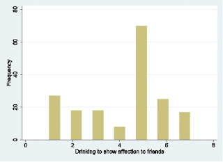
Instead of doing it manually (copy and paste), we can do it much quicker: if you want to save a histogram graph:

1) hist d1, freq
2) graph export d1.eps, replace
3) graphout d1.eps using example.rtf
4) Open file example.rtf, you will see this:

The only problem is that it is not clear as we use Excel. 
Always use Excel if the graph is simple. If it is more complicated, use Stata's graphic functions.

Checking for autocorrelation /serial correlation

What is autocorrelation?
1) So you have an equation to predict values of a dependent variable Y….
2) The predicted values (Y’i)  are only ‘close’ the the real values (Yi)….
3) The difference between predicted and real values are called by different names: residual (the left over), or error term (the part that equation cannot predict)
4) There are two important assumptions related to the residual/error term: – they should not correlate with each other, and their variance should be constant.
5) If the first assumption is violated, or the residuals (between different waves of data, or different groups) correlate with each other, we have autocorrelation. This is particularly so in time series data analysis (called ‘serial correlation’)
6) If the second assumption is violated, we have the phenomenon called heteroskedasticity
How to check for them?
How to know if the first assumption is violated?
We can set the data as panel data, then use Wooldridge test as following in Stata
xtserial DEP (list of predictor)  ------> if p value smaller than 0.05, assumption is violated. If I have d1 as DEP and age is the only predictor,

xtserial d1 age

Wooldridge test for autocorrelation in panel data
H0: no first-order autocorrelation
    F(  1,       1) =      0.059
           Prob>| F| =      0.8486

-->This indicates there is no autocorrelation

Another way is to do this: set the data as times series, then

reg DEP (list of predictor)

dwstat

How to know if heterokesdasticity exist?

reg DEP var list

estat hett

Breusch-Pagan / Cook-Weisberg test for heteroskedasticity
         Ho: Constant variance
         Variables: fitted values of d3

         chi2(1)      =     0.73
         Prob >|chi2|  =   0.3942

-->This indicates no heterokesdascity

What do to?
What to do if you find autocorrelation? Remove its effect by:

prais d1 age, corc

Iteration 0:  rho = 0.0000
Iteration 1:  rho = 0.0795
Iteration 2:  rho = 0.0808
Iteration 3:  rho = 0.0808
Iteration 4:  rho = 0.0808

Cochrane-Orcutt AR(1) regression -- iterated estimates

      Source |       SS       df       MS              Number of obs =     127
-------------+------------------------------           F(  1,   125) =    4.85
       Model |  14.3667947     1  14.3667947           Prob >| F|      =  0.0295
    Residual |  370.582352   125  2.96465882           R-squared     =  0.0373
-------------+------------------------------           Adj R-squared =  0.0296
       Total |  384.949147   126  3.05515196           Root MSE      =  1.7218

------------------------------------------------------------------------------
          d1 |      Coef.   Std. Err.      t    P>|t|     [95% Conf. Interval]
-------------+----------------------------------------------------------------
         age |   .0306289   .0139136     2.20   0.030     .0030922    .0581656
       _cons |   3.001655   .5507311     5.45   0.000     1.911689     4.09162
-------------+----------------------------------------------------------------
         rho |   .0808052
------------------------------------------------------------------------------
Durbin-Watson statistic (original)    1.838574
Durbin-Watson statistic (transformed) 2.000578

What do do if you find heteroskedasticity?
Heteroskedasticity can distort  estimations. In stata, we remove its effect by using robust regression
reg Y X, robust

 reg d1 age, robust

Linear regression                                      Number of obs =     128
                                                       F(  1,   126) =    5.55
                                                       Prob>| F|      =  0.0201
                                                       R-squared     =  0.0409
                                                       Root MSE      =   1.722

------------------------------------------------------------------------------
             |               Robust
          d1 |      Coef.   Std. Err.      t    P>|t|     [95% Conf. Interval]
-------------+----------------------------------------------------------------
         age |   .0322989   .0137162     2.35   0.020      .005155    .0594428
       _cons |   2.945031   .5509205     5.35   0.000     1.854776    4.035286
------------------------------------------------------------------------------

Typical cup

Non-parametric tests

1) Test for normality: Kolmogorov-Smirnov one-sample test

2) Comparing two related samples: Wilcoxon Signed Ranks Test

3) Comparing two unrelated samples: Mann-Whitney U-Test (both variables are categorical, ranksum2 in Stata)

4) Comparing more than two related samples: The Friedman Test

5) Comparing more than two unrelated samples: the Kruska-Wallis H-Test (kwallis2 in Stata)

6) Comparing variables of ordinal or dichotomous scales: Spearman Rank-Order (both variables are ordinal, spearman in Stata), Point-Biserial (pbis in Stata), Biserial (if one is ordinal, one is continuous) Correlations

7) Tests for nominal scale data: Chi-square and Fisher Exact Tests

Checking for multivariate normality

 

When we run a multiple regression, we assume that the predictors in our model are normally distributed. Not each of them! But the combination of them is normally distributed. That is called ‘multivariate normality’.

We, again, need to check for that. In the Z table, we note that data points that lie below –3 standard deviations or above +3 standard deviations would mean ‘outliers’ because they are too far from the mean (3 sd). Conventionally, we can use these points (-3: +3) to say which observations are ‘out of the range’ when we consider multivariate normality.

 

What we need to do now is to combine all predictors and see which points are outliers. This task is extremely difficult, unless we use a computer program called biplot.

 

We now see that observations 8, 265, 266 are potentially outliers, though they are not out of the range. We may delete them if our sample size is large enough, or keep them since these outliers are not severe.

Basic nonparametric tests in Stata

There are many variables that do not follow the rule of normal distributions. We may call them ‘qualitative’, ‘discrete’ or ‘categorical’ variables. What to do ? Consider the following cases

1) One continuous variable to be compared across 2, 3 groups or more? And you want to do something like ANOVA ?
If alcohol is an index, if it is a continuous variable following normal distribution, and you would like to compare alcohol across 4 groups (numbered from 1 to 4 in variable ‘ex’):
anova alcohol i.ex
pwcompare i.ex
--------------------------------------------------------------
             |                                 Unadjusted
             |   Contrast   Std. Err.     [95% Conf. Interval]
-------------+------------------------------------------------
          ex |
    2 vs 1  |    7.84005   .6146453       6.63063     9.04947
     3 vs 1  |   1.063768   .7986802     -.5077717    2.635308
     4 vs 1  |   11.31003   .7748954      9.785287    12.83477
     3 vs 2  |  -6.776282   .8104726     -8.371025   -5.181539
    4 vs 2  |   3.469976   .7870442      1.921332     5.01862     4 vs 3  |   10.24626   .9378378      8.400902    12.09161--------------------------------------------------------------
Yellow lines indicate significant differences. But if it is clearly that, as an index, alcohol does not follow normal distribution? We should think about rank.

kwallis2 alcohol, by(ex)
(where alcohol is a continuous variable, not normally distributed)
One-way analysis of variance by ranks (Kruskal-Wallis Test)
ex       Obs   RankSum  RankMean
--------------------------------
  1      115   9896.00     86.05
  2      104  22142.00    212.90
  3       45   4775.00    106.11
  4       49  12328.00    251.59
Chi-squared (uncorrected for ties) =   178.123 with    3 d.f. (p = 0.00010)
Chi-squared (corrected for ties)   =   191.758 with    3 d.f. (p = 0.00010)
Multiple comparisons between groups
-----------------------------------
(Adjusted p-value for significance is 0.004167)
Ho: alcohol(ex==1) = alcohol(ex==2)
    RankMeans difference =    126.85  Critical value =     32.31
    Prob = 0.000000 (S)
Ho: alcohol(ex==1) = alcohol(ex==3)
    RankMeans difference =     20.06  Critical value =     41.98
    Prob = 0.103737 (NS)
Ho: alcohol(ex==1) = alcohol(ex==4)
    RankMeans difference =    165.54  Critical value =     40.73
    Prob = 0.000000 (S)
Ho: alcohol(ex==2) = alcohol(ex==3)
    RankMeans difference =    106.79  Critical value =     42.60
    Prob = 0.000000 (S)
Ho: alcohol(ex==2) = alcohol(ex==4)
    RankMeans difference =     38.69  Critical value =     41.37
    Prob = 0.006809 (NS)
Ho: alcohol(ex==3) = alcohol(ex==4)
    RankMeans difference =    145.48  Critical value =     49.30
    Prob = 0.000000 (S)

2) Compare two groups?
Two-sample Wilcoxon rank-sum (Mann-Whitney) test
ranksum2 bin, by(sex)
Two-sample Wilcoxon rank-sum (Mann-Whitney) test
         sex |      obs    rank sum    expected
-------------+---------------------------------
      Female |       39      2518.5      3607.5
        Male |      145     14501.5     13412.5
-------------+---------------------------------
    combined |      184       17020       17020
unadjusted variance    87181.25
adjustment for ties   -25532.48
                     ----------
adjusted variance      61648.77
Ho: bin(sex==Female) = bin(sex==Male)
             z =  -4.386
    Prob > |z| =   0.0000
U/mn         .69257294
3) Association between two categorical variables?
spearman bin sex, stats(rho p)
Number of obs =     184
Spearman's rho =       0.3242
Test of Ho: bin and sex are independent
    Prob > |t| =       0.0000
4) Regression with many variables?
logistic bin sex ethnic

Beaten to death in Vietnam: Security camera captured insecurity in Hanoi

 

This man was beaten for One Hour long in his own apartment in the capital city (Hanoi) of Vietnam. Two security cameras, inside and outside of the apartment, recorded everything.

His neighbours called the police many times. But they only came after the punishment was complete.

The man was hospitalized afterward, with several injuries in his eyes and other parts of the body.

The young woman who led the gangster men to his apartment used to work with him in a company. They had not met for four years because during that time she was prison due to a criminal activity.

This video together with its story was posted on laodong.com.vn – an electronic news agency that aims to serve ‘the labourers’.

The agency however, only posted the video, without any comments, though in the latter part of the video, it asks ‘Was the police too late?’ . This attitude reflects the fact that all news agencies in Vietnam are heavily controlled by the state. Editors have to find ways to ‘break the fence’ without risking their own lives.

Hanoi Region (purple area)

Không đề

Vợ bắt về nằng nặc

Thầy bỗng dưng nghiêm khắc

Bạn bè sinh phản trắc

Ý nào cũng thấy tắc!

‘Market song’: from begging to ‘cultural heritage’

A traditional music performance which is said to belong to the ordinary people begging in cities for a living. Songs and music are often performed at an open market’s corner. Audience drop coins/notes in front of performers. This performance disappeared in 1990s when Vietnam’s economy became better and the number of people begging in cities reduced. Now, artists are revitalizing it, turning it into a ‘cultural heritage’.

Vietnam music tradition

Vietnam music tradition

What is publication?

Publication is making a content available to the general public.

A journal article, or book, is called a publication. A conference paper, or working paper, is in principle a publication. Sometimes, a conference paper may get cited many times. A piece of ‘scientific information’ posted on a blog can be seen as a ‘publication’ (in this sense, you can publish everyday!)

But peer reviewed journal articles are always preferred to other forms.

A list of publications is often a requirement to applying for academic positions.

Once published, the content is not always available to the public. Users have to pay a fee in order to download an article. Many people discontent with that. They initiate ‘free access’, ‘open’ web-based stores in order to make a publication really ‘public’.

This can be an example. Second example, the one that contains several hundreds of books from various sources. The second example is here. The third is here. I strongly recommend the second.

All possible models

This interesting command allows an exploration of all possible models

In STATA only.

allpossible modelcmd depvar varlist [if exp] [in range] [weight] , {
               eclass(statistics_list) | rclass(progname statistics_list) } [ detail
               npmax(#) format(format) cellwidth(#) modelcmd_options]

How to run a logistic regression in STATA?

When: outcome follows binomial distribution (two values, 0 and 1)
The nature: Outcome values are converted to logits – the distribution is approximately Gaussian (normal)
Assumptions: Linearity between converted outcome values and independent variables, no outliers that may distort estimates, goodness of fit (p is larger than 0.05, basically means the set of predictors can predict well the outcome, or not (p is smaller than 0..05))
IN STATA:
1. Key command:
logit DEPVAR INDVARLIST, or
2. Check for linearity:
boxit: logit
If the results indicate that a predictor is nonlinearly associated with the outcome (p<.05), transform it, or recode it.
3. Check for outliers:
predict res, dx
tw (scatter res DEPVAR)
Outliers are values far away from the main ‘cloud’ of others. Remove them.
4. Check for goodness of fit: do this when two others have been done
estat gof, group(10)
5. Re-run the final model to get estimates.
Report Odd ratios: Understand the meaning of Odds and Odds ratios
For example if you have a predictor sex (male=1, female=0), and an outcome cancer, an estimate for sex =1.2, what does it mean?
It means: the probability of getting cancer among sampled men / probability of getting cancer among sampled women=1.2, or
The probability of getting cancer among sampled men is 1.2 times the probability of getting cancer among sampled women, when all other factors (education, occupation, etc.) are equal.
6. (This is not required but if you like): Take the 'margin' probability: If you want to know what the probability that being a man, 40 years old, manual labourer has done xyz in the last week, when all other factors are the same, then you should you margins function in Stata.
margins, at(female=0 age=40 jobtype=1) atmeans
marginsplot, noci

http://feeds.feedburner.com/blogspot/sGXLS